
Cats or Dogs!?
Today we will use Tensorflow machine learning models to cats and dogs images!
Key Imports
import os # for file path manipulation
# machine learning library for data pipeline,
# data manipulation, layer design, and model creation
import tensorflow as tf
from tensorflow.keras import utils, datasets, layers, models
import numpy as np # numeric manipulation
import pandas as pd # data frame manipulation
from matplotlib import pyplot as plt # plotting
Getting Data
We will read in the data set from Google API
# location of data
_URL = 'https://storage.googleapis.com/mledu-datasets/cats_and_dogs_filtered.zip'

# download the data and extract it
path_to_zip = utils.get_file('cats_and_dogs.zip', origin=_URL, extract=True)

# construct paths
PATH = os.path.join(os.path.dirname(path_to_zip), 'cats_and_dogs_filtered')
train_dir = os.path.join(PATH, 'train')
validation_dir = os.path.join(PATH, 'validation')

# parameters for data sets
BATCH_SIZE = 32
IMG_SIZE = (160, 160)

# construct train and validation datasets
train_dataset = utils.image_dataset_from_directory(train_dir,
                                                   shuffle=True,
                                                   batch_size=BATCH_SIZE,
                                                   image_size=IMG_SIZE)

validation_dataset = utils.image_dataset_from_directory(validation_dir,
                                                        shuffle=True,
                                                        batch_size=BATCH_SIZE,
                                                        image_size=IMG_SIZE)

# construct the test dataset by taking every 5th observation out of the validation dataset
val_batches = tf.data.experimental.cardinality(validation_dataset)
test_dataset = validation_dataset.take(val_batches // 5)
validation_dataset = validation_dataset.skip(val_batches // 5)
Visualizing Data
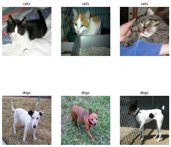
The following function prints out six images in two rows, three cats and three dogs, from the first batch of train_dataset.
def cat_dog_plotter():
    # Get the class names ["cats", "dogs"]
    class_names = train_dataset.class_names
    plt.figure(figsize=(10, 10))
    for images, labels in train_dataset.take(1):
      # Get the first three indices of cat images
      cat_ind = np.flatnonzero(np.array(labels) - 1)[:3]
      # Get the first three indices of dog images
      dog_ind = np.flatnonzero(np.array(labels))[:3]
      # Concatenate for looping
      ind = np.concatenate((cat_ind, dog_ind), axis = None)
    for i in range(6):
      # Designate 6 total plots
      ax = plt.subplot(2, 3, i + 1)
      # Plot the image
      plt.imshow(images[ind[i]].numpy().astype("uint8"))
      # Provide the classification label
      plt.title([n for n in class_names for c in range(3)][i])
      # No X and Y axis printed for the images
      plt.axis("off")

cat_dog_plotter()
Check Label Frequencies
# labels iterator
labels_iterator= train_dataset.unbatch().map(lambda image, label: label).as_numpy_iterator()
# We loop through the iterator and record the number of occurences
# of 0s (cats) and 1s (dogs)
class_dict = {0:0, 1:0}
for i in list(labels_iterator):
  class_dict[i] = class_dict[i] + 1
class_dict
The resulting dictionary is {0: 1000, 1: 1000}. We have a training data set of 2000 images, half of which are cats and the others are dogs. Thus a model of always predicting cats or always predicting dogs would be our initial model, with an expected accuracy of 50% (coin-toss chance)
Model 1
Using two 2D convolution layers, two MaxPooling2D layers, one drop out, one flatten, and two dense layers, we train for just shy of 3 million parameters.
# Model construction
model1 = models.Sequential([
                           layers.Conv2D(32, (3, 3), activation='relu', input_shape=(160, 160, 3)),
                           layers.MaxPooling2D((2, 2)),
                           layers.Conv2D(32, (3, 3), activation='relu'),
                           layers.MaxPooling2D((2, 2)),
                           layers.Dropout(0.2, seed = 11235),
                           layers.Flatten(), # flatten to 1D
                           layers.Dense(64, activation='relu'),
                           layers.Dense(2) # number of classes in your data set
])
# Compile the model by specifying optimizer and loss function
model.compile(optimizer='adam',
              # No softmax layer
              loss = tf.keras.losses.SparseCategoricalCrossentropy(from_logits=True),
              # Show  accuracy during training process
              metrics = ['accuracy'])

history = model1.fit(train_dataset,
                    epochs = 20, # how many rounds of training to do
                    validation_data = validation
)
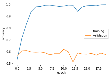
The training accuracy is consistently between 0.98 and 0.99. The validation accuracy is consistently around 0.61.
Comparing this result to the baseline, we would say this is a moderate increase in terms of raw percentage (~11%), but it certainly is a nontrivial improvement in terms of practical significance as our model actually now is better than randomly guessing (with ~50% accuracy)
There is definitely overfitting. The training accuracy starts with the higher end of 0.8 right off th start of epoch 1, and often can climb up to 0.99 during runs by the end. The validation accuracy certainly has never crossed the 0.8 threshold, indicating significant overfitting in model1.
Model 2 (Data Augmentation)
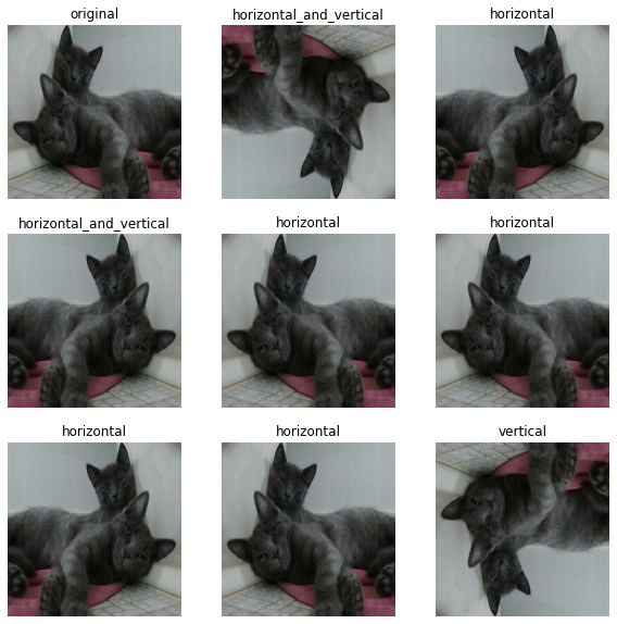
Demonstrating RandomFlip
for image, _ in train_dataset.take(1):
  plt.figure(figsize=(10, 10))
  first_image = image[0]
  # Allowed flip types
  flip_types = ['horizontal', 'vertical', "horizontal_and_vertical"]
  for i in range(9):
    ax = plt.subplot(3, 3, i + 1)
    if i == 0:
      plt.imshow(first_image / 255)
      plt.title("original")
      plt.axis('off')
    else:
      flip_choice = random.choice(flip_types)
      # Randomy choose a flip style
      # and randomly execute (may not flip)
      data_augmentation = tf.keras.layers.RandomFlip(flip_choice)
      augmented_image = data_augmentation(tf.expand_dims(first_image, 0))
      plt.imshow(augmented_image[0] / 255)
      plt.title(flip_choice)
      plt.axis('off')
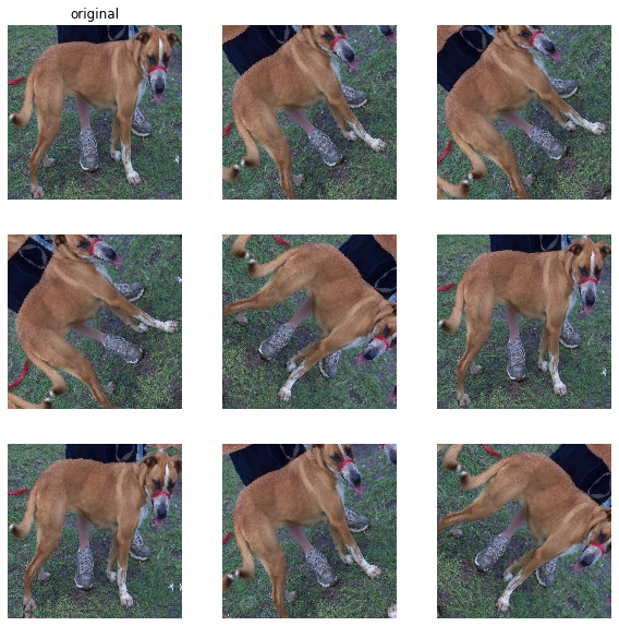
Demonstrating RandomRotation
for image, _ in train_dataset.take(1):
  plt.figure(figsize=(10, 10))
  first_image = image[0]
  for i in range(9):
    ax = plt.subplot(3, 3, i + 1)
    if i == 0:
      plt.imshow(first_image / 255)
      plt.title("original")
      plt.axis('off')
    else:
      data_augmentation = tf.keras.layers.RandomRotation(
          # Rotating randomly between [-20% * 2pi, 30% * 2pi]
          factor = 0.2,
          # The input is extended by reflecting about the edge of the last pixel.
          fill_mode='reflect',
          interpolation='nearest'
      )
      augmented_image = data_augmentation(tf.expand_dims(first_image, 0))
      plt.imshow(augmented_image[0] / 255)
      plt.axis('off')
# Model construction
model2 = models.Sequential([
                            layers.RandomFlip(mode = 'horizontal_and_vertical',
                                              input_shape=(160, 160, 3)),
                            layers.RandomRotation(factor = 0.2,
                                                  fill_mode='reflect',
                                                  interpolation='nearest'),
                            layers.Conv2D(32, (3, 3), activation='relu'),
                            layers.MaxPooling2D((2, 2)),
                            layers.Conv2D(32, (3, 3), activation='relu'),layers.MaxPooling2D((2, 2)),
                            layers.Dropout(0.2, seed = 11235),
                            layers.Flatten(),
                            layers.Dense(64, activation='relu'),
                            layers.Dense(2) # number of classes in your dataset
                            ])
model2.compile(optimizer='adam',
               loss = tf.keras.losses.SparseCategoricalCrossentropy(from_logits=True), # no softmax layer
               metrics = ['accuracy'])

history = model2.fit(train_dataset,
                     epochs = 20,
                     validation_data = validation_dataset
)
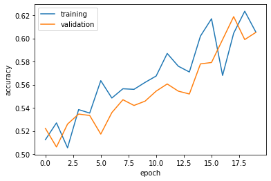
The training accuracy have been stable between 0.60 and 0.65, with the validation accuracy hitting as high as 0.6943 and as low as 0.5767.
The overall training accuracy is much worse than that of model1, but the validation accuracy is similar. This is a good sign, in fact, in terms of lack of overfitting.
We see that the training and validation accuracies are now much more aligned, indicating that random rotation and flipping introduced forced our model to not over-focus on the specific noises and instead focus on larger patterns that discern cats from dogs.
Model Three (Data Preprocessing)
By letting a data preprocessor handle the scaling prior to the training process, we can spend more of our training energy handling actual signal in the data and less energy having the weights adjust to the data scale.
# Preprocessor
i = tf.keras.Input(shape=(160, 160, 3))
x = tf.keras.applications.mobilenet_v2.preprocess_input(i)
preprocessor = tf.keras.Model(inputs = [i], outputs = [x])
# Model construction
model3 = models.Sequential([preprocessor,
                            layers.RandomFlip(mode = 'horizontal_and_vertical'),
                            layers.RandomRotation(factor = 0.2,
                                                  fill_mode='reflect',
                                                  interpolation='nearest'),
                            layers.Conv2D(32, (3, 3), activation='relu'),
                            layers.MaxPooling2D((2, 2)),
                            layers.Conv2D(32, (3, 3), activation='relu'),layers.MaxPooling2D((2, 2)),
                            layers.Dropout(0.2, seed = 11235),
                            layers.Flatten(),
                            layers.Dense(64, activation='relu'),
                            layers.Dense(2) # number of classes in your dataset
                            ])
model3.compile(optimizer='adam',
               loss = tf.keras.losses.SparseCategoricalCrossentropy(from_logits=True), # no softmax layer
               metrics = ['accuracy'])

history = model3.fit(train_dataset,
                     epochs = 20,
                     validation_data = validation_dataset
)

The validation accuracy of the model was consistently between 0.72 and 0.76.
The training accuracies actually are the lowest so far, with only about 0.52, but the validation accuracies are consistently above 0.70, easily beating model1 and model2.
There is no indication of overfitting. If anything, the low training accuracy and high validation accuracy means that the model struggled with the training data because it only looked for general patterns. After 20 epochs, however, the model has learned crucial patterns that allowed it to successfully predict our validation set with high accuracy.
Model 4 (Transfer Learning)
Here we take advantage of an existing machine learning model and incorporate it as a layer in out model
# Download and configure MobileNetV2 as a layer for our own model
IMG_SHAPE = IMG_SIZE + (3,)
base_model = tf.keras.applications.MobileNetV2(input_shape=IMG_SHAPE,
                                               include_top=False,
                                               weights='imagenet')
base_model.trainable = False

i = tf.keras.Input(shape=IMG_SHAPE)
x = base_model(i, training = False)
base_model_layer = tf.keras.Model(inputs = [i], outputs = [x])
# Model construction
model4 = models.Sequential([preprocessor,
                            layers.RandomFlip(mode = 'horizontal_and_vertical'),
                            layers.RandomRotation(factor = 0.2,
                                                  fill_mode='reflect',
                                                  interpolation='nearest'),
                            #base_model_layer, # MobileNetV2 that we downloaded
                            layers.Conv2D(64, (3, 3), activation='relu'),
                            layers.Dense(64, activation='relu'),
                            layers.Dense(2)
                            ])
model4.summary()

The training accuracy oscillates between 0.90 and 0.92, whereas the validation accuracy is consistently around 0.97!
This result is significantly better than our initial model1 (which achieved only about 60% accuracy on the validation data set)
We do not observe any concerning overfitting. The training and validation accuracies remain close during the multiple runs of model training and cross-validation processes.
Score on Test Data
We use model4 to predict the labels of the test_dataset
y_pred = model4.predict(test_dataset)
labels_pred = y_pred.argmax(axis=1)
predicted = labels_pred
We then get the true labels from the dataset
true_labels = np.empty(0)
for _, label in test_dataset:
  for i in label:
    true_labels = np.append(true_labels, i)
true_labels = true_labels.astype(int)
To calculate the accuracy, we calculate the percentage of matches
np.mean(predicted == true_labels)
After several trials, the final test accuracy remains stuck around 0.52, which is surprising given our high performance on the validation data set.This tells us once again that the raw test data set may contain novel patterns or outlier patterns that are not present in the training (or even the validation data set), thus our model may not get the opportunity to observe and learn about these during the training/validation process.